Digital Signal Processing
Copyright © 1999, 2002, 2007 Kees Krijnen.
The setup of a simple dynamic laser light scattering DSP system (fig.1) consist of:
- A conversion of a light detector analog signal into digital information, in the form of a sequence of binary numbers. This involves two operations: sampling and analog-to-digital (A/D) conversion.
- Perform numerical operations on the digital information by special-purpose digital hardware or PC. In this case the operations are spectrum analysis, "analog" autocorrelation, or both simultaneously.
- Display DSP process on PC monitor continuously.
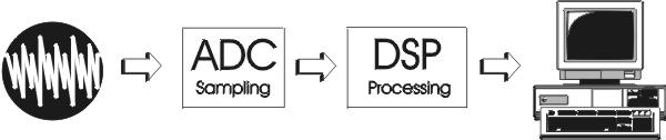
Fig. 1
To facilitate digital processing, a continuous-time signal must be converted to a sequence of numbers [REF1]. Sampling is essentially a selection of a finite number of data at any finite time interval as representatives of the infinite amount of data contained in the continuous-time signal in that interval. Sampling is the fundamental operation of digital signal processing, and avoiding (or at least minimizing) aliasing is the most important aspect of sampling. Aliasing is the fundamental distortion introduced by sampling. Aliasing causes the digitized pattern not look like the analog signal digitized. If analog signals at higher frequencies are present, the sampling process will produce sum and difference frequencies, in particular, will produce spurious low-frequency signals - in the signal passband - that cannot be distinguished from the signal. The Nyquist criterion provides a correct reconstruction of the analog signal, stated by Shannon's reconstruction theorem. Reconstruction is the operation of converting a sampled signal back to a continuous-time signal. Aliasing is caused by sampling at a lower rate than the Nyquist rate for the given signal.
Nyquist rate: sampling frequency ≥ 2 times highest frequency signal or noise component
Analog noise in data-acquisition systems take three basic forms [REF5]: transmitted noise, inherent in the received signal, device noise, generated within the devices used in data acquisition (preamps, converters, etc.), and induced noise, `picked up' from the outside world, power supplies, logic, or other analog channels, by magnetic, electrostatic, or galvanic coupling.
Noise is either random or coherent (i.e., related to some noise-inducing phenomenon within or outside the system). Random noise is usually generated within components, such as resistors, semiconductor junctions, or transformer cores, while coherent noise is either locally generated by processes, such as modulation/demodulation, or coupled-in. Coherent noise often takes the form of `spikes', although it may be of any shape.
The finite resolution of the A/D conversion process introduces `quantization noise', which may be thought of as either a truncation (or roundoff) error, or as a `digitizing' noise, depending on the context.
Noise is characterized in terms of either root-mean-square (rms) or peak-to-peak measurements, within a stated bandwidth. Noise leads to random errors and missing codes in an ADC. Since these errors can lead to a closed-loop system making inappropriate responses to specific false data points, high-resolution systems, where random noise tends to limit resolution and to cause errors, can benefit by digital or analog filtering to smooth the data.
If higher frequencies signal or noise than the Nyquist rate are part of the analog signal, a low-pass filter must be applied to match the Nyquist criterion.
Spectral Analysis
The departure point for a discussion of spectral analysis is the Fourier transform equation pair [REF5]:
Fourier Transform 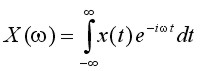
Inverse Fourier Transform 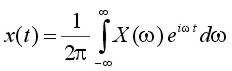
where t is time, ω is angular frequency (2πf), x(t) is the signal - a function of time - and X(ω) is its counterpart in the frequency (spectral) domain. These equations give us, at least formally, the mechanics for taking a signal' time-domain representation and resolving it into its spectral weights - called Fourier coefficients. The Fourier series is a trigonometric series F(f) by which we may approximate some arbitrary function f(t) or x(t) - real world signal [REF3]. Specifically, F(f) is the series (another way to describe above frequency-domain function X(ω)):
F(t) = A0 + A1Sin(t)+ B1Cos(t) + A2Sin(2t) + B2Cos(2t) + ... + AnSin(nt) + BnCos(nt)
eiωt = Cos(ωt) + iSin(ωt)
In the limit as n (i.e. the number of terms) approaches infinity, the trigonometric series is equal to the real world signal. It means that any real world signal can be considered as a composite waveshape which can be breaked down into its component sinusoids. A0, A1, B1, ...and An, Bn, are the Fourier coefficients. When the Fourier coefficients are known the time-domain function x(t) can be easily calculated - reconstructed - by summation of the component sinusoids. Since the Fourier equations require continuous integrals, they have only indirect bearing on digital processors. However, under certain circumstances, a sampled (digitized) signal can be related faithfully to its Fourier coefficients through the discrete Fourier transform (DFT):
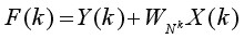
(Forward) DFT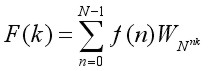
Inverse DFT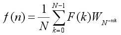
| where: | F(k) = frequency components or transform f(n) = time base data points or inverse transform N = number of data points n = discrete times, 0 to N-1 k = discrete frequencies, 0 to N-1 WN = e-i2π/N = Cos(2π/N) - iSin(2π/N) |
Provided that the signal is sampled frequently enough (Nyquist rate), and assuming that the signal is periodic, the above DFT equations hold exactly. What is most interesting from the standpoint of DSP is that the DFT equation provides us with a means to estimate spectral content by digitizing an incoming signal and simply performing a series of multiply/accumulate operations.
A process is required that can isolate, or `detect' any single harmonic (sine wave) component within a complex waveshape [REF3]. To be useful quantitatively, it will have to be capable of measuring the amplitude and phase of each harmonic component. While measuring any harmonic component of a composite wave, all of the other harmonic components must be ignored.
According to Fourier the way to detect and measure a sine wave component within a complex waveshape is to multiply through by a unit amplitude sine wave of the identical frequency and then find the average value of the resultant. The two functions must have the same number of data points, corresponding domains, etc. The reason this works is that both sine waves are both positive at the same time, and both negative at the same time, so that the products of these two functions will have a positive average value. Since the average value of a sinusoid is normally zero, the original digitized sine wave has been `rectified' or `detected'. This scheme will work for any harmonic component, changing the frequency of the unit amplitude sine wave to match the frequency of the harmonic component being detected. The same approach will work for the cosine components if the unit sine function is replaced with a unit cosine function.
Orthogonality is the method used to extract the sinusoid being analyzed while ignoring all other sinusoidal components [REF4]. Orthogonality implies that if one sinusoidal is multiplied by another, an average value of zero will obtained (averaged over any number of full cycles), if either:
- the sinusoids are dephased by 90° or,
- the sinusoids are integer multiple frequencies.
It is necessary to deal with full cycles of a sinusoid for the average value to be zero. This requirement can be satisfied by scaling the frequency term so that exactly one full sinusoid fits into the domain of the function working with.
The composite waveform is generated by summing in harmonic components:
| F(t) = A0 + A1Sin(t)+ B1Cos(t) + A2Sin(2t) + B2Cos(2t) + ... + AnSin(nt) + BnCos(nt) |
If this composite function is multiplied by Sin(Kt) (or, alternatively, Cos(Kt)), where K is an integer, the following terms on the right hand side of the equation are created:
| A0Sin(Kt) + A1Sin(t)Sin(Kt) + B1Cos(t)Sin(Kt) + ... + AkSin2(Kt) + BkCos(Kt)Sin(Kt) + ... + AnSin(nt)Sin(Kt) + BnCos(nt)Sin(Kt) |
Treating each of these terms as individual functions, if argument (Kt) equals the argument of the sinusoid it multiplies, that component will be `rectified'. Otherwise, the component will not be rectified. From what is shown above, two sinusoids of ± 90° phase relationship (i.e. Sine/Cosine), or integer multiple frequency, represent orthogonal functions. As such, when summed over all values within the domain of definition, they will all yield a zero resultant (regardless of whether they are handled as individual terms of combined into a composite waveform). This is precisely what is demanded from a procedure to isolate the harmonic components of an arbitrary waveform.
The DFT algorithm consist of stepping trough the digitized data points of the input time-domain function, multiplying each point by sine and cosine functions, and summing the resulting products into accumulators (one for the sine component and one for the cosine). When every point has been processed in this manner, the accumulators (i.e. the sum-totals of the preceding process) is divided by the number of data points. The resulting quantities are the average values for the sine and cosine components at the frequency being investigated as described above. This process must be repeated for all integer multiple frequencies up to the frequency that is equal to the sampling rate minus 1 (i.e. twice the Nyquist frequency minus 1).
If the digitized matrix f(t) is considered to be a row matrix, the process can be described as a matrix multiplication [REF6,7]:
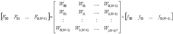
WN = e-i2π/N = Cos(2π/N) - iSin(2π/N)
The DFT WNN square coefficient matrix is called the array of Twiddle Factors. One is needed for the Sine function and one for the Cosine function.
Unfortunately, the large number of multiplications required by the DFT limits its use in real-time signal processing. The computational complexity of the DFT grows with the square of the number of input points; to resolve a signal of length N into N spectral components F(k) requires N2 complex multiplications (4N2 real multiplications). Given the large number of input points needed to provide acceptable spectral resolution, the computational requirements of the DFT are prohibitive for most applications. For this reason, tremendous effort was devoted to developing more efficient ways of computing the DFT. This effort produced the fast Fourier transform (FFT) invented by Cooley and Tukey (1965). The FFT uses mathematical shortcuts to reduce the number of calculations the DFT requires.
The DFT (and FFT) requirement to deal with full cycles of a sinusoid rises inevitably the need for a high-pass filter. The frame length and timing of data acquisition determines the low cut-off frequency. The Nyquist criterion requires a low-pass filter, under experimental conditions this means a band-pass filter has to be applied to the input signal.
One-Dimensional FFT
Suppose an N-point DFT is accomplished by performing two N/2 -point DFTs and combining the outputs of the smaller DFTs to give the same output as the original DFT. The original DFT requires N2 complex multiplications and N2 complex additions. Each DFT of N/2 input samples requires (N/2)2 = N2/4 multiplications and additions, a total of N2/2 calculations for the complete DFT. Dividing the DFT into two smaller DFTs reduces the number of computations by 50 percent. Each of these smaller DFTs can be divided in half, yielding N/4 -point DFTs. If we continue dividing the N-point DFT calculation into smaller DFTs until we have only two-point DFTs, the number of complex multiplications and additions is reduced to Nlog2N. For example, a 1024-point DFT requires over a million complex additions and multiplications. A 1024-DFT divided down into two-point DFTs needs fewer than ten thousand complex additions and multiplications, a reduction of over 99 percent!
Dividing the DFT into smaller DFTs is the basis of the FFT. A radix-2 FFT divides the FFT into two smaller DFTs, each of which is divided into two smaller DFTs, and so on, resulting in a combination of two-point DFTs. The radix-2 Decimation-In-Time (DIT) FFT divides the input time-domain sequence into two groups, one of even samples and the other of odd samples. N/2-point DFTs are performed on these sub-sequences, and their outputs are combined to form the N-point DFT.
The input time-domain sequence in equation (1), is divided into even and odd sub-sequences to become the equation:
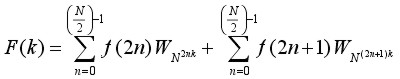 (2)
(2)
By substitution equation (2) becomes:
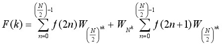 (3)
(3)
By substitution equation (3) can also be expressed as two equations:
 (4.1)
(4.1)
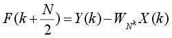 (4.2)
(4.2)
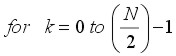
Together these equations (4.1) and (4.2) form an N-point FFT. Each of these two equations can be divided to form two more. The final decimation occurs when each pair of equations together computes a two-point DFT (one point per equation). The pair of equations that make up the two-point DFT is called a radix-2 `butterfly' (fig. 2). The butterfly is the core calculation of the FFT. The entire FFT is performed by combining butterflies in patterns determined by the FFT algorithm based on the Similarity, Shifting, Addition and Stretching transform theorems. An array of 2n data points yields n stages of computation in FFT.
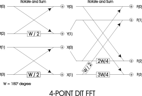
fig. 2
In general, the input of FFTs are assumed to be complex. When input is purely real - for example, in case of digitized analog data - their symmetric properties compute the DFT very efficiently [REF9].
One such optimized real FFT algorithm is the packing algorithm. The original 2N-point real input sequence is packed into an N-point complex sequence. Next, an N-point FFT is performed on the complex sequence. Finally the resulting N-point complex output is unpacked into the 2N-point complex sequence, which corresponds to the DFT of the original 2N-point real input.
Using this strategy, the FFT size can be reduced by half, at the FFT cost function of N operations to pack the input and unpack the output. Thus, the real FFT algorithm computes the DFT of a real input sequence almost twice as fast as the general FFT algorithm.
The TMS320C542 (see PALS Experimental Setup chapter) real FFT algorithm is a radix-2, DIT DFT algorithm in four phases:
In phase 1 - packing and bit-reversal of real input - the input is bit-reversed so that the output at the end of the entire algorithm is in natural order. First, the original 2N-point real input sequence is copied into contiguous sections of memory and interpreted as an N-point complex sequence. The even-indexed real inputs form the real part of the complex sequence and the odd-indexed real inputs form the imaginary part. This process is called packing. Next, this complex sequence is bit-reversed and stored into the data processing buffer.
In phase 2 - N-point complex FFT - an N-point complex DIT FFT is performed in place in the data-processing buffer. The twiddle factors are in Q15 format and are stored in two separate tables, pointed to by sine and cosine. Each table contains 512 values, corresponding to angles ranging from 0 to almost 180 degrees. The indexing scheme used in this algorithm permits the same twiddle tables for inputs of different sizes.
Phase 3 - separation of odd and even parts - separates the FFT output to compute four independent sequences, which are the even real, odd real, even imaginary, and the odd imaginary parts.
Phase 4 - generation of final output - performs one more set of butterflies to generate the 2N-point complex output, which corresponds to the DFT of the original 2N-point real input sequence.
Often, the last stage in a FFT spectral analysis is the computation of the power spectrum from the frequency-domain transform of the input time-domain sequence.
The power spectrum is a meaningful way of representing random signals in the frequency domain by their mean-square value or energy content. Now from Parseval's theorem [REF10]:
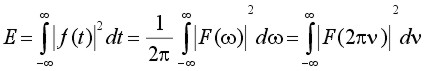 (5)
(5)
where ω = 2πν and ν is expressed in Hertz. Equation (5) states that the energy content of f(t) is given by 1/(2π) times the area under the |F(ω)|2 curve. For this reason, the quantity |F(ω)|2 is called the power spectrum or energy spectral density of f(t).