Autocorrelation
Copyright © 1999, 2002, 2007 Kees Krijnen.
Autocorrelation gives an indication to what degree the time signal f(t) is similar to a displaced (delayed) version of itself as a function of the displacement. This technique is - for example - used for the detection of echoes in the signal (radar, sonar) or detection of periodic signals buried in random noise (LDV, ELS). The autocorrelation function is defined by [REF10]:
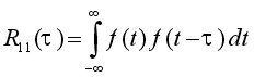 (6)
(6)
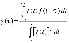
Sometimes, a normalized quantity γ(τ) defined by
 (7)
(7)
is also called the autocorrelation function of f(t). In this case it is clear that γ(0) = 1. The average autocorrelation function of periodic signals of period T are also periodic with the same period. This does not mean that autocorrelation function of a periodic signal will have the same waveshape as the signal autocorrelated. The autocorrelation of a sine wave is a cosine waveshape [REF10]. This means when looking for a periodic sinusoid signal in random noise the autocorrelation function will show a cosine waveshape mixed with the autocorrelation function of the random noise.
The basics of a digital hardware correlator are shown by means of reviewing an existing correlator IC device from TRW LSI Products Inc. (fig. 3). This device has been designed not only for auto- or crosscorrelation, but also for pattern and character recognition, video frame synchronization, bar code identification, radar signature recognition etc.
The TRW TMC2023 is an monolithic 64-bit correlator with a 7-bit three-state buffered digital output. This device consist of three 64-bit independently clocked shift registers, one 64-bit reference holding latch, and a 64-bit independently clocked digital summing network. The device is capable of a 30MHz parallel correlation rate.
The 7-bit threshold register allows the user to preload a binary number from 0 to 64. Whenever the correlation is equal to or greater than the number in the threshold register, the threshold flag goes HIGH.
The 64-shift mask register (M register) allows the user to mask or selectively choose `no compare' bit positions enabling total word length flexibility. In case of autocorrelation this mask register is used for the undelayed clocked signal.
The summing process is initiated when the comparison result between the A register and R latch (NXOR-gate) is clocked into the summing network by a rising edge of CLK S. Typically, CLK A and CLK S are tied together so that a new correlation score is computed for each new alignment of the A register and the R latch. Every clock cycle the contents of register n is shifted to register n+1. When LDR goes HIGH, the contents of register B are copied into the R latch. With LDR low, a new template may be entered serially into register B, while parallel correlation takes place between register A and the R latch.
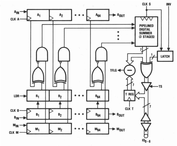
fig. 3. Functional block diagram TMC2023 (courtesy TRW LSI Products. Inc.).
In case of a 1x1-bit autocorrelator function, shift registers B and M - tied together - are used for the undelayed signal. CLK A, CLK B, CLK M and CLK S are also tied together. Input AIN is held HIGH, filling register A with ones. Every clock cycle BIN and MIN are shifted into B1 and M1, and register Bn and Mn are shifted into Bn+1 and Mn+1. Every 64-clock cycles register B is copied into the R latch by a LDR HIGH pulse - an external clock counter circuit is needed, which resets every 64-clock cycles and gives the LDR pulse. After this copy action latch register R is n clock cycles delayed compared to register M until the clock counter equals 64, loads register B into the R latch, and resets again. The AND-gate acts as a 1x1-bit multiplier of register R (delayed B) and M, multiplication - equation (6) - is required. The output IO0-6 gives the summing of the 64-channel 1x1-bit autocorrelation every clock cycle of the delayed signal.
A microprocessor keeps track of the autocorrelation process over multiple 64-clock cycles. Every clock cycle the microprocessor reads the summing result IO0-6 and the contents of the clock counter. The summing result is added to an array indexed by the clock counter. This array gives the integrated 64-channel 1x1-bit autocorrelation function over a finite period of time.
The scheme for a nxn multi-bit autocorrelator is exactly the same. The shift registers are n multi-bit shift registers. The latch register is a n multi-bit latch register. Instead of an AND-gate a nxn multiplier device is required.
The first PCS autocorrelators were 1x1-bit correlators. Ideally the PMT light detector electronics generates one digital pulse for each photon the PMT receives what makes the light detection truly digital. The 1x1-bit correlators were perfectly suited to correlate the PMT digital pulse train. However, this meant that the autocorrelation clock rate should be higher or equal to the digital pulse rate. In practice this requirement is not easily achieved. The correlation clock rate - sample time - is set to a value to maximize autocorrelation resolution. If more than one pulse is received within the sample time overflow occurs. Prescaling or multi-bit correlation avoids clipping of the digital input signal. Nowadays, PCS autocorrelators are multi-bit correlators allowing prescaling if necessary, offer multiple simultaneous correlation sample times, or even logarithmic sample times.
The implementation of autocorrelation by means of a DSP microprocessor is almost directly derived from equation (6). A frame of N data points is acquired continuously and stored into a circular buffer of size N. The last acquired data point overwrites the first - oldest - one. Between successive samples, the last acquired data point - f(0) - is multiplied with itself and with the previous N-1data points. The multiplication results are added to an array of size N, indexed by the number of data points difference between the last data point and the previous N-1 data points. The array contents indexed by 0 to (N-1) gives the integrated autocorrelation function.
To find a periodic signal burried in the signal f(t), the Fourier
transform  of the autocorrelation
function is computed, which is called the energy spectrum density of
f(t). If f(t) is a real function, then the autocorrelation function
R11(τ) and the energy spectral density
|F(ω)|2 constitute a Fourier transform pair [REF10]; that is,
of the autocorrelation
function is computed, which is called the energy spectrum density of
f(t). If f(t) is a real function, then the autocorrelation function
R11(τ) and the energy spectral density
|F(ω)|2 constitute a Fourier transform pair [REF10]; that is,
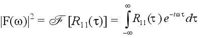 (8)
(8)
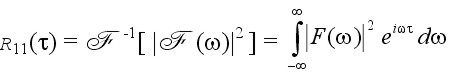
This result is known as the Wiener-Khintchine theorem.
The number of autocorrelation channels of a DSP microprocessor correlator is limited by the time available for the multiplication process between successive samples. If the energy spectrum is computed simultaneously - by means of FFT - the time available, and so the number of autocorrelation channels is even more limited. Another restricting factor is that the FFT computation requires a log2 number of data points. It limits the autocorrelation resolution by forcing the number of autocorrelation channels also bound to log2, even if there is computation time left to setup more autocorrelation channels.
Photon Correlation Spectroscopy
Classic - static - light scattering is concerned with the average intensity of the scattered light and its dependence on both the concentration and size of scattering particles, and the scattering angle. The intensity of scattered light depends inverse fourth power on wavelength (Raleigh, 1871) and sixth power on radius of particle.
For particles less than 1/10th of wavelength of the illuminating beam, the scattering is isotropic, equal energy is scattered at all angles - Raleigh theory. Mie theory (1908) describes exactly how particles of different sizes and optical properties interact with light and is used to analyze light scattering of particles above 1/10th of wavelength. Mie theory approximation computing algorithms have an upper limit due to (optical parameter) ill-conditioning [REF11]. Above this limit Anomalous Diffraction and Fraunhofer Diffraction approximations [REF12] can be used. References [REF11], [REF12] and [REF13] are excellent, comprehensive papers on static light scattering by particles.
Intensity Fluctuation Spectroscopy - dynamic light scattering - is concerned with the amplitude modulation of the scattered light. In case of an illuminated suspended sample, the modulation is caused by interference of scattered light due to the Brownian movement of the suspended particles. Brownian motion (Brown, 1828) is the random movement of suspended particles due to collision with the random thermal motion of solvent molecules (Einstein, 1905). If the suspended particle is big compared to the solvent molecules those movements will be small. Smaller particles will move faster, due to the greater influence of the solvent molecules.
Interference occurs because of the different path lengths traversed by light scattered from different particles. The illuminating beam must be coherent, that means light waves must be parallel and in phase. Lasers produce coherent, monochromatic light. The temporal fluctuations of interest appear in one coherence area, and the signal-to-noise ratio does not increase when more than one coherence area is detected. The intensity of a coherence area will be seen to vary as dark and light patches interchanging in the field of view. The rate of these fluctuations is determined by the speed of the diffusing particles - related to particle size, shape, and medium viscosity and temperature.
A coherence area could be defined as the coherently illuminated minimum volume resulting maximum intensity modulation by interference. Intensity modulation will minimize - intensity of scattered light becomes constant - when the viewed area is too large (incoherent). Ideally, one coherence area is viewed, depending on quality of optics and sensitivity of light detector.
The rate of the intensity fluctuations vary with speed of diffusing particles and are random, no distinctive sinusoid can be detected. Although, autocorrelation does not extract sinusoids from the intensity fluctuations, the correlatorgram shows an exponential curve. The rate of decay is related to the diffusion coefficient of the suspended particles. Autocorrelation detects similarity of the scattering signal in time, and this similarity will be lost sooner when particles move faster - are smaller - thus resulting a faster decay of the exponential correlation curve.
Generally, a photon multiplier tube (PMT) is used as a light detector. These are photo emissive devices coupled with electron multipliers. When a photon strikes the photocathode, an electron is emitted and multiplied by sequential dynodes. The multiplier sections have typical gains of 106 so that a measurable current is produced at the anode. In a photon counting system the pulses resulting from - ideally single - photons are selected, amplified and correlated, hence the name Photon Correlation Spectroscopy (PCS).
The autocorrelation of the scattered electric field E of the incident light and the frequency components of the intensity signal form a Fourier transform pair - equation (8). When the autocorrelation of E is known, the frequency components can be computed. Detectors, e.g. PMTs, respond to the intensity I rather than the electric field of incident light. In general, the autocorrelation of I [G2(τ) - second order] is not simply related to autocorrelation of E [G1(τ) - first order]; however, if E(t) is a Gaussian random variable the Siegert relation gives
G2(τ) = I 2 + |G1(τ)|2
By substitution the normalized second order autocorrelation function becomes
G2(τ) = 1 + Ce-τt (9)
| where: | τ = 2DτK2 C = experimental constant correlator Dτ = diffusion coefficient K =  λ = wavelength of laser Φ = scattering angle n = refractive index suspending liquid |
Gaussian random means that the number of particles contributing to the intensity modulation of scattered light should be significant and Gaussian distributed. In experimental conditions this viewed number should be at least one hundred. The Stokes-Einstein equation for diffusion of a monosized sample states:
Dτ = 
| where: | k = Boltzmann's constant T = absolute temperature η = viscosity of the solvent d = spherical particle diameter |
Thus, using PCS, average size of monodispersed spherical samples can be determined based on first principles. The size distribution determination of polydispersed samples is a lot more difficult; (1) different polydisperse size distributions can give similar autocorrelation results, and (2) intensity depends sixth power on radius, bigger particles contribute more to the signal than smaller ones. A more extensive treatment of PCS theory can be found in reference [REF2].
Frequency determination for light scattered from particles in uniform motion are conceptually simpler than for diffusing particles. Laser Doppler Velocimetry (LDV) is a well established technique in engineering for the study of fluid flows. Two laser beams in phase are caused to cross at a particular point in the measurement cell. The lens in the receiver optics - a coherent detector - is focussed at the center of this crossing point. At the intersection of the laser beams, Young's [REF14] interference fringes are formed of known spacing given by the simple equation
 (10)
(10)
Particles moving through this fringe pattern scatter light what gives rise to a sinusoidal intensity modulation at the detector whose frequency can be measured and thus the related velocity calculated by multiplying S with found frequency. The frequency is determined by a Fourier transform - equation (8) - of the autocorrelation function, which also gives the autocorrelation due to scattered light by the Brownian movement of suspended particles. The latter autocorrelation function is, in respect to LDV, background noise.
The following experiment is setup as a LDV experiment. The results can be applied to Electrophoretic Light Scattering (ELS). The essence of an ELS system is a cell with electrodes at either end to which a potential gradient is applied. Charged particles move towards the appropriate electrode through the crossing point of the laser beams, their velocity is measured and expressed in unit field strength as their mobility. The stability of suspended particles, emulsions, are strongly influenced by the electrical charges that exist at the particle liquid surface.
The term Laser Doppler Velocimetry is - however in the past established in publications like [REF2] - not a correct description of the physical phenomena. LDV was originally setup as a low angle single laser beam experiment where the laser beam crossed high speed particles like those ejected out of a jet fighter exhaust. Those high speed particles indeed caused a doppler shift of the laser light frequency. When two laser beams in phase were crossed the same term was still used, however in this case for low speed particles the sinusoidal intensity modulation delivers the information. The term Phase Analysis Laser Scattering (PALS) is applied when one of the laser beams is modulated.